ML model to predict future offtake
Introduction
This is the analysis I did for a part of the interview when I applied Danone, I submitted this analysis with in 24 hours.
Description: We have historical sales ( column: target in the excel file) from 2015-01-01 to 2020-09-01 for 8 product SKU (BRANDA1,BRANDA2,BRANDA3,BRANDA4,BRANDB1,BRANDB2,BRANDB3,BRANDB4),as well as other information that may help, column sales1, sales2, marketing1, marketing2, category1, category2 ( Columns names are anonymized,e.g., sales1 means sales related information1)
Purpose: Implement exploratory data analysis and forecast future 12 month(from 2020-10-01 to 2021-09-01) for each SKU.
import pandas as pd
import numpy as np
import matplotlib.pyplot as plt
import seaborn as sns
import sklearn.tree as st
from sklearn.ensemble import RandomForestRegressor
from sklearn.model_selection import train_test_split
from pathlib import Path
data_dir = Path('data')
df= pd.read_csv(filepath_or_buffer ='interview_test.csv')
EDA
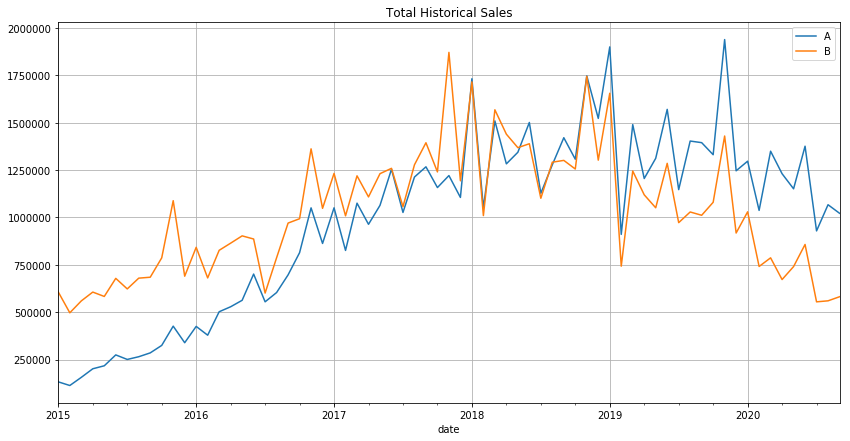
Firstly, take a look at the total sales of brand A and brand B from 2015 to 2020. The most interesting fact is that before 2018, B’s sales was higher than A’s but since then, A’s sales exceeded B. We can do furthr research to investigate why this happened. Both A and B’s sales grew steadily from 2015, but incurred a severe drop in 2020, which was due to the COVID-19 probably. We can also observe that at the end of every year, there is a peak in total sales, this is because of the “shopping festival” on Nov,11th。
A = df[df['brand'] == 'BRANDA'].reset_index()
B = df[df['brand'] == 'BRANDB'].reset_index()
data1 = pd.DataFrame({"date":A['date'],
    "A":A['target'],
            "B":B['target'],
        }).dropna(axis = 0)
data1['date'] = pd.to_datetime(data1['date'])
a = (data1.groupby('date').sum())[['A','B']]
a.plot(figsize = (14,7),grid = True)
plt.title('Total Historical Sales')
Text(0.5, 1.0, 'Total Historical Sales')
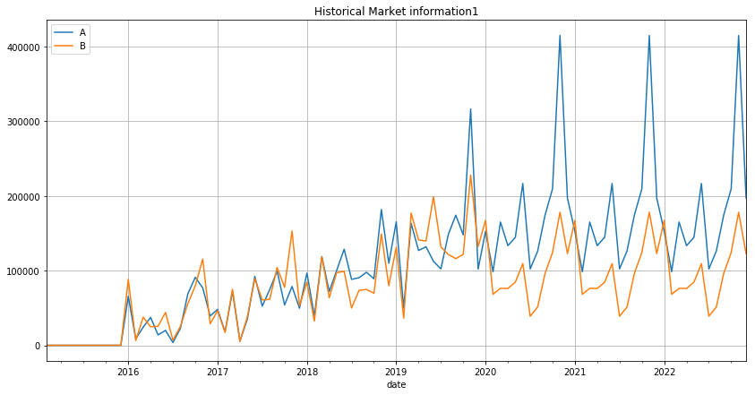
Then we look at the curve of “marketing 1” of A and B. A and B have the same trend of marketing1 throughout the period. And marketing 1 reached its peak on Nov,11th every year, which is in line with the behavior of the sales. Therefore, we may make a hypothesis that higher marketing1 leads to higher sales. And we can simply run a regression to verify this. Here I do not show the process.
data1 = pd.DataFrame({"date":A['date'],
    "A":A['marketing1'],
            "B":B['marketing1'],
        }).dropna(axis = 0)
data1['date'] = pd.to_datetime(data1['date'])
a = (data1.groupby('date').sum())[['A','B']]
a.plot(figsize = (14,7),grid = True)
plt.title('Historical Market information1')
Text(0.5, 1.0, 'Historical Market information1')
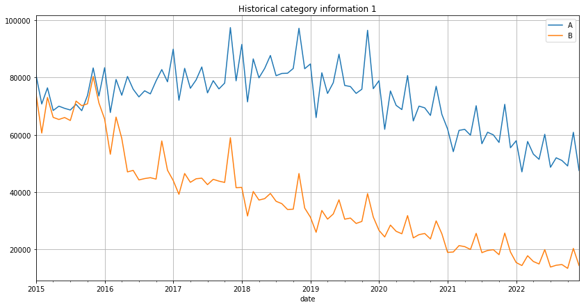
The curve of historical category1 shows that A’s category1 is pretty stable up to now but intends to decrease in the future. In contrast, B is continuously decreasing the category1 starting from 2016. May be this is one factor which results in the different sales performance between A and B
data1 = pd.DataFrame({"date":A['date'],
    "A":A['category1'],
            "B":B['category1'],
        }).dropna(axis = 0)
data1['date'] = pd.to_datetime(data1['date'])
a = (data1.groupby('date').sum())[['A','B']]
a.plot(figsize = (14,7),grid = True)
plt.title('Historical category information 1')
Text(0.5, 1.0, 'Historical category information 1')
If we look at the sales of A and B in detail, we can observe that almost all sales of products of brand A exceed brand B’s after 2018. And the trend within each kind of product is pretty the same
A1 = df[df['sku'] == 'BRANDA1'].reset_index()
A2 = df[df['sku'] == 'BRANDA2'].reset_index()
A3 = df[df['sku'] == 'BRANDA3'].reset_index()
A4 = df[df['sku'] == 'BRANDA4'].reset_index()
B1 = df[df['sku'] == 'BRANDB1'].reset_index()
B2 = df[df['sku'] == 'BRANDB2'].reset_index()
B3 = df[df['sku'] == 'BRANDB3'].reset_index()
B4 = df[df['sku'] == 'BRANDB4'].reset_index()
data1 = pd.DataFrame({"date":A1['date'],
    "A1":A1['target'],
            "A2":A2['target'],
         "A3":A3['target'],
         "A4":A4['target'],
         "B1":B1['target'],
         "B2":B2['target'],
         "B3":B3['target'],
         "B4":B4['target'],
        }).dropna(axis = 0)
data1['date'] = pd.to_datetime(data1['date'])
a = (data1.groupby('date').sum())[['A1','A2','A3','A4','B1','B2','B3','B4']]
a.plot(figsize = (14,7),grid = True)
plt.title('Historical Sales for Each Products')
Text(0.5, 1.0, 'Historical Sales for Each Products')
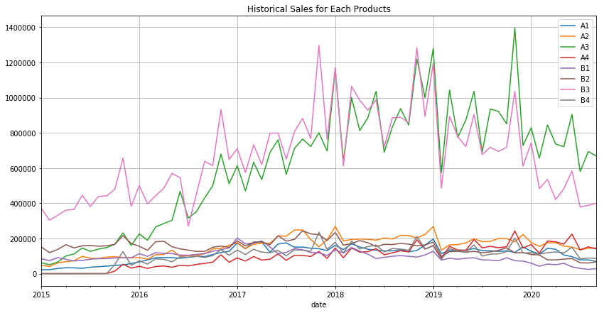
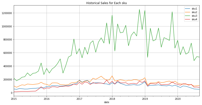
The curve below indicates that the sales trends between different kinds of products are not homogeneous. Therefore, I will do the further analysis on each kind of products, say SKU1 SKU2 SKU3 and SKU4, and train 4 model on these four kinds of data and do the prediction seperately.
sku1 = df[(df['sku'] == 'BRANDA1')|(df['sku'] == 'BRANDB1')].reset_index()
sku2 = df[(df['sku'] == 'BRANDA2')|(df['sku'] == 'BRANDB2')].reset_index()
sku3 = df[(df['sku'] == 'BRANDA3')|(df['sku'] == 'BRANDB3')].reset_index()
sku4 = df[(df['sku'] == 'BRANDA1')|(df['sku'] == 'BRANDB4')].reset_index()
data1 = pd.DataFrame({"date":sku1['date'],
    "sku1":sku1['target'],
            "sku2":sku2['target'],
         "sku3":sku3['target'],
         "sku4":sku4['target']
        }).dropna(axis = 0)
data1['date'] = pd.to_datetime(data1['date'])
a = (data1.groupby('date').mean())[['sku1','sku2','sku3','sku4']]
a.plot(figsize = (14,7),grid = True)
plt.title('Historical Sales for Each SKU')
Text(0.5, 1.0, 'Historical Sales for Each sku')
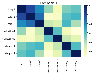
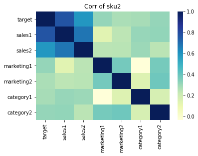
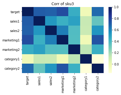
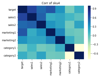
Plots below depict the correlation between each variable within each SKU.
The sales of all kinds of products are positively correlated with ‘sales1’ and ‘sales2’.
However, the correlation between sales and other 4 features is pretty low for SKU1 and SKU2.
In SKU3 and SKU4, the correlation is more significant, especially for marketing1 and category1.
sns.heatmap(sku1.drop(['index'],axis = 1).corr(),cmap="YlGnBu")
plt.title('Corr of sku1')
plt.show()

sns.heatmap(sku2.drop(['index'],axis = 1).corr(),cmap="YlGnBu")
plt.title('Corr of sku2')
plt.show()

sns.heatmap(sku3.drop(['index'],axis = 1).corr(),cmap="YlGnBu")
plt.title('Corr of sku3')
plt.show()

sns.heatmap(sku4.drop(['index'],axis = 1).corr(),cmap="YlGnBu")
plt.title('Corr of sku4')
plt.show()
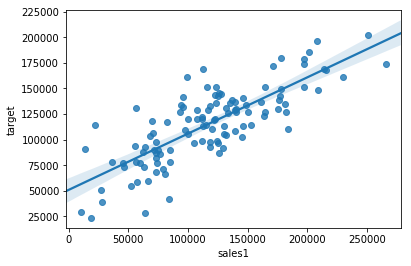
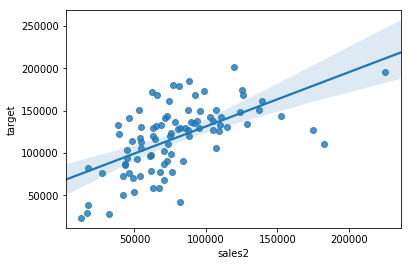
To see the relationship between sales information and sales clearly, Scatterplots of sales vs sales information are shown bellow. The straight line is a fitted line of the data using linear regression. I only show the result of SKU1 since the result is the same for SKU2 3 and 4.
From the plot, we can see that both sales information 1 and sales information 2 are positively related to our target data. Unfortunately, we don’t have future values for these two features to do the forecast.
sns.regplot(x="sales1", y="target", data=sku1)
plt.show()
sns.regplot(x="sales2", y="target", data=sku1)
plt.show()
Model Fitting and Forecasting
(Note: I first choose a model to predict SKU1 products and show the detailed modeling process, then predict the target value for brandA1 and brandB1. For SKU2 3 and 4, I use the model chosen for SKU1, and train the model by the new data and make the prediction. Here I use category1, category2, marketing1 and marketing2 as features.
SKU1
Choose the data where the column of “sku” is “brandA1” or “brandB1”, the date is from 2016/1/1 to 2020/9/1 as our training data. Drop the rows with NA or 0. Then I split the data in the ratio of 0.75:0.25 so that we can use cross validation to choose the model.
a = sku1[sku1['date'] == '2016/1/1'].index
b = sku1[sku1['date'] == '2020/9/1'].index
c = sku1.loc[range(a[0],b[0]+1),['date','target','marketing1','marketing2','category1','category2']].dropna(axis = 0)
Train = c[c != 0].dropna(axis = 0)
Trainx = Train.drop(['date','target'],axis = 1)
Trainy = Train['target']
train_x, test_x, train_y, test_y = train_test_split(c.drop(["target",'date'],axis=1), c["target"], test_size=0.25, random_state=42)
Decision Tree
Firstly, grow a simple tree where the depth is set from 1 to 20, and the MSE curve of training and test are plotted.
train_err = []
test_err = []
for i in range(1,21,1):
    model = st.DecisionTreeRegressor(criterion='mse',max_depth = i)
    model.fit(train_x,train_y)
    predict = model.predict(train_x)
    train_err.append(sum((predict - train_y)**2/len(predict)))
    predict = model.predict(test_x)
    test_err.append(sum((predict - test_y)**2)/len(predict))
plt.plot(range(1,21,1),train_err)
plt.plot(range(1,21,1),test_err)
plt.title("Mean Squared Error")
plt.legend(["train","test"])
<matplotlib.legend.Legend at 0x1b364d0cc0>
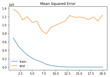
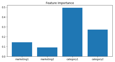
From the plot, the test MSE is minimized when depth = 7 or 8, and the training error decreases as depth increases. Therefore, I set the depth to be 8 and train the model with the whole data. We can see that the feature ‘category1’ is the most important one, which is in line with our observation in the correlation within SKU1
model = st.DecisionTreeRegressor(criterion='mse',max_depth = 8)
model.fit(Trainx,Trainy)
fig = plt.figure(figsize=(8,4))
importance = model.feature_importances_
plt.bar([x for x in range(len(importance[0:4]))], importance[0:4])
plt.xticks(range(4),train_x.columns)
plt.title("Feature Importance")
Text(0.5, 1.0, 'Feature Importance')
Random Forest
Since the test error in Decision Tree is not satisfying, I apply the random forest. I set the number of trees from 1 to 100. Since we have a dominated feature “category1”, I set the max features within each tree to be 2 so that they will not be correlated with each other.
train_err = []
test_err = []
for i in range(1,151,1):
    model = RandomForestRegressor(n_estimators=i,max_features=2)
    model.fit(train_x,train_y)
    predict = model.predict(train_x)
    train_err.append(sum((predict - train_y)**2/len(predict)))
    predict = model.predict(test_x)
    test_err.append(sum((predict - test_y)**2)/len(predict))
plt.plot(range(1,151,1),train_err)
plt.plot(range(1,151,1),test_err)
plt.title("Mean Squared Error")
plt.legend(["train","test"])
<matplotlib.legend.Legend at 0x1b368b0860>
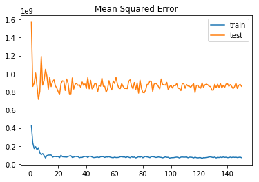
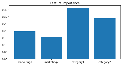
This time the test error drops while the training error is close to zero. And I set the number of trees to be 80 and retrain the model with full data. Now the feature importances are averaged.
model = RandomForestRegressor(n_estimators=80,max_features=1)
model.fit(Trainx,Trainy)
fig = plt.figure(figsize=(8,4))
importance = model.feature_importances_
plt.bar([x for x in range(len(importance[0:4]))], importance[0:4])
plt.xticks(range(4),train_x.columns)
plt.title("Feature Importance")
Text(0.5, 1.0, 'Feature Importance')
Prediction
Choose the data where the column ‘sku’ is ‘brandA1’ and the date is from 2020/10/1 to 2021/9/1. Then we have the data for predicting the target sales of A1. Same process for B1. Then make the prediction.
a = A1[A1['date'] == '2020/10/1'].index
b = A1[A1['date'] == '2021/9/1'].index
A1_data = A1.loc[range(a[0],b[0]+1),['marketing1','marketing2','category1','category2']]
a = B1[B1['date'] == '2020/10/1'].index
b = B1[B1['date'] == '2021/9/1'].index
B1_data = B1.loc[range(a[0],b[0]+1),['marketing1','marketing2','category1','category2']]
A1_data
.dataframe tbody tr th {
    vertical-align: top;
}

.dataframe thead th {
    text-align: right;
}
A1_target = model.predict(A1_data)
B1_target = model.predict(B1_data)
So our ultimate model is random forest
SKU2
a = sku2[sku2['date'] == '2016/1/1'].index
b = sku2[sku2['date'] == '2020/9/1'].index
c = sku2.loc[range(a[0],b[0]+1),['date','target','marketing1','marketing2','category1','category2']].dropna(axis = 0)
Train = c[c != 0].dropna(axis = 0)
Trainx = Train.drop(['date','target'],axis = 1)
Trainy = Train['target']
a = A2[A2['date'] == '2020/10/1'].index
b = A2[A2['date'] == '2021/9/1'].index
A2_data = A2.loc[range(a[0],b[0]+1),['marketing1','marketing2','category1','category2']]
a = B2[B2['date'] == '2020/10/1'].index
b = B2[B2['date'] == '2021/9/1'].index
B2_data = B2.loc[range(a[0],b[0]+1),['marketing1','marketing2','category1','category2']]

model = RandomForestRegressor(n_estimators=80,max_features=1)
model.fit(Trainx,Trainy)

A2_target = model.predict(A2_data)
B2_target = model.predict(B2_data)
SKU3
a = sku3[sku3['date'] == '2016/1/1'].index
b = sku3[sku3['date'] == '2020/9/1'].index
c = sku3.loc[range(a[0],b[0]+1),['date','target','marketing1','marketing2','category1','category2']].dropna(axis = 0)
Train = c[c != 0].dropna(axis = 0)
Trainx = Train.drop(['date','target'],axis = 1)
Trainy = Train['target']
a = A3[A3['date'] == '2020/10/1'].index
b = A3[A3['date'] == '2021/9/1'].index
A3_data = A3.loc[range(a[0],b[0]+1),['marketing1','marketing2','category1','category2']]
a = B3[B3['date'] == '2020/10/1'].index
b = B3[B3['date'] == '2021/9/1'].index
B3_data = B3.loc[range(a[0],b[0]+1),['marketing1','marketing2','category1','category2']]

model = RandomForestRegressor(n_estimators=80,max_features=1)
model.fit(Trainx,Trainy)

A3_target = model.predict(A3_data)
B3_target = model.predict(B3_data)
SKU4
a = sku4[sku4['date'] == '2016/1/1'].index
b = sku4[sku4['date'] == '2020/9/1'].index
c = sku4.loc[range(a[0],b[0]+1),['date','target','marketing1','marketing2','category1','category2']].dropna(axis = 0)
Train = c[c != 0].dropna(axis = 0)
Trainx = Train.drop(['date','target'],axis = 1)
Trainy = Train['target']
a = A4[A4['date'] == '2020/10/1'].index
b = A4[A4['date'] == '2021/9/1'].index
A4_data = A4.loc[range(a[0],b[0]+1),['marketing1','marketing2','category1','category2']]
a = B4[B4['date'] == '2020/10/1'].index
b = B4[B4['date'] == '2021/9/1'].index
B4_data = B4.loc[range(a[0],b[0]+1),['marketing1','marketing2','category1','category2']]

model = RandomForestRegressor(n_estimators=80,max_features=1)
model.fit(Trainx,Trainy)

A4_target = model.predict(A4_data)
B4_target = model.predict(B4_data)
Results
results = (pd.DataFrame(np.vstack((A1_target,A2_target,A3_target,A4_target,B1_target,B2_target,B3_target,B4_target)))).T
results.columns = ['A1','A2','A3','A4','B1','B2','B3','B4']
results.to_csv(r"Predicted_targets.csv",index=True,header=True)