Predicting interest rates at the Lending Club

Load and prepare the data

We start by loading the data to R in a dataframe.

lc_raw <- read_csv("data/LendingClub Data.csv",  skip=1) %>%  #since the first row is a title we want to skip it. 
  clean_names() # use janitor::clean_names()

ICE the data: Inspect, Clean, Explore

glimpse(lc_raw[, 1:10])

## Rows: 42,538
## Columns: 10
## $ int_rate    <dbl> 0.05, 0.05, 0.05, 0.05, 0.05, 0.05, 0.05, 0.05, 0.05, 0.05…
## $ loan_amnt   <dbl> 8000, 6000, 6500, 8000, 5500, 6000, 10200, 15000, 14750, 1…
## $ term_months <dbl> 36, 36, 36, 36, 36, 36, 36, 36, 36, 36, 36, 36, 36, 36, 36…
## $ installment <dbl> 241.3, 181.0, 196.0, 241.3, 165.9, 181.0, 307.6, 452.4, 44…
## $ dti         <dbl> 2.11, 5.73, 17.68, 22.71, 5.75, 21.92, 18.62, 9.72, 18.32,…
## $ delinq_2yrs <dbl> 0, 0, 0, 0, 0, 0, 0, 0, 0, 0, 0, 0, 0, 0, 0, 0, 0, 0, 0, 0…
## $ annual_inc  <dbl> 50000, 52800, 35352, 79200, 240000, 89000, 110000, 135000,…
## $ grade       <chr> "A", "A", "A", "A", "A", "A", "A", "A", "A", "A", "A", "A"…
## $ emp_title   <chr> NA, "coral graphics", NA, "Honeywell", "O T Plus, Inc", "F…
## $ emp_length  <chr> "5 years", "< 1 year", "n/a", "n/a", "10+ years", "2 years…

lc_clean<- lc_raw %>%
  dplyr::select(-x20:-x80) %>% #delete empty columns
  filter(!is.na(int_rate)) %>%   #delete empty rows
  mutate(
    issue_d = mdy(issue_d),  # lubridate::mdy() to fix date format
    term = factor(term_months),     # turn 'term' into a categorical variable
    delinq_2yrs = factor(delinq_2yrs) # turn 'delinq_2yrs' into a categorical variable
  ) %>% 
  dplyr::select(-emp_title,-installment, -term_months, everything()) #move some not-so-important variables to the end. 


glimpse(lc_clean[, 1:10])

## Rows: 37,869
## Columns: 10
## $ int_rate            <dbl> 0.05, 0.05, 0.05, 0.05, 0.05, 0.05, 0.05, 0.05, 0.…
## $ loan_amnt           <dbl> 8000, 6000, 6500, 8000, 5500, 6000, 10200, 15000, …
## $ dti                 <dbl> 2.11, 5.73, 17.68, 22.71, 5.75, 21.92, 18.62, 9.72…
## $ delinq_2yrs         <fct> 0, 0, 0, 0, 0, 0, 0, 0, 0, 0, 0, 0, 0, 0, 0, 0, 0,…
## $ annual_inc          <dbl> 50000, 52800, 35352, 79200, 240000, 89000, 110000,…
## $ grade               <chr> "A", "A", "A", "A", "A", "A", "A", "A", "A", "A", …
## $ emp_length          <chr> "5 years", "< 1 year", "n/a", "n/a", "10+ years", …
## $ home_ownership      <chr> "MORTGAGE", "MORTGAGE", "MORTGAGE", "MORTGAGE", "M…
## $ verification_status <chr> "Verified", "Source Verified", "Not Verified", "Ve…
## $ issue_d             <date> 2011-09-01, 2011-09-01, 2011-09-01, 2011-09-01, 2…

The data is now in a clean format stored in the dataframe “lc_clean.”

# Build a histogram of interest rates. Make sure it looks nice!
lc_clean %>% 
  ggplot(aes(x = int_rate)) +
    geom_histogram(bins = 20) +
    labs(title = "The majority of loans are taken with an interest rate of around 10%",
         subtitle = "Histogram of loan interest rates",
         x = "Interest Rate",
         y = "Count") +
  scale_x_continuous(labels = scales::percent) + # change labels
  theme_solarized()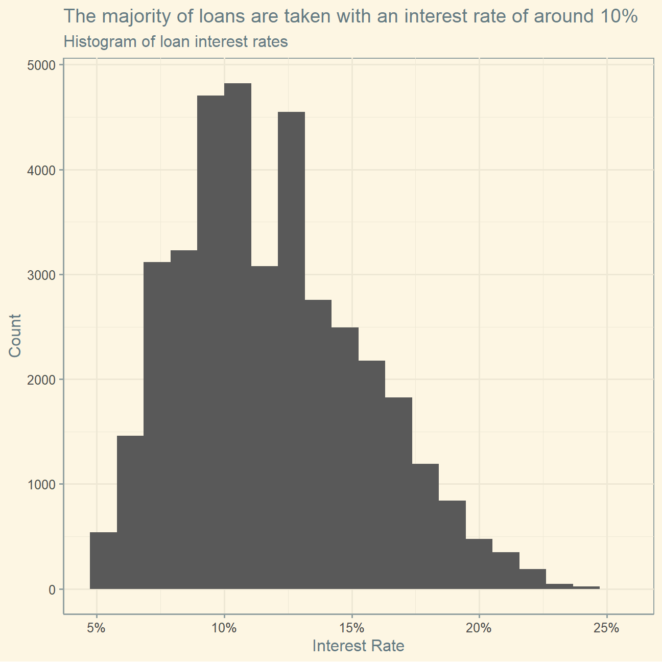

# Build a histogram of interest rates but use different color for loans of different grades 
lc_clean %>% 
  ggplot(aes(x = int_rate, fill = grade)) +
    geom_histogram(bins = 20) +
    labs(title = "The loan grade lets us group loans by interest rate",
         subtitle = "Histogram of loan interest rates colored by grade",
         x = "Interest Rate",
         y = "Count",
         fill = "Grade") +
    scale_x_continuous(labels = scales::percent) + # change labels
    theme_solarized()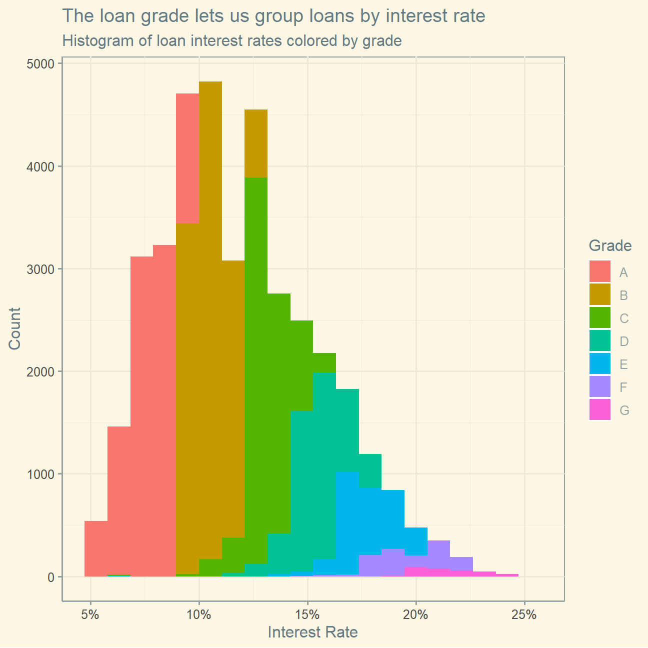

# Produce a scatter plot of loan amount against interest rate and add visually the line of best fit
lc_clean %>% 
  ggplot(aes(x = loan_amnt, y = int_rate)) +
    geom_point(alpha = 0.3) + # reduce opacity to improve readability
    geom_smooth() +
    scale_x_continuous(labels = scales::dollar) + # change labels x
    scale_y_continuous(labels = scales::percent) + # change labels y
    labs(title = "The best-fit line indicates a positive correlation",
         subtitle = "Scatterplot of loan amount and interest rate with best-fit line",
         x = "Loan Amount",
         y = "Interest Rate") +
    theme_solarized()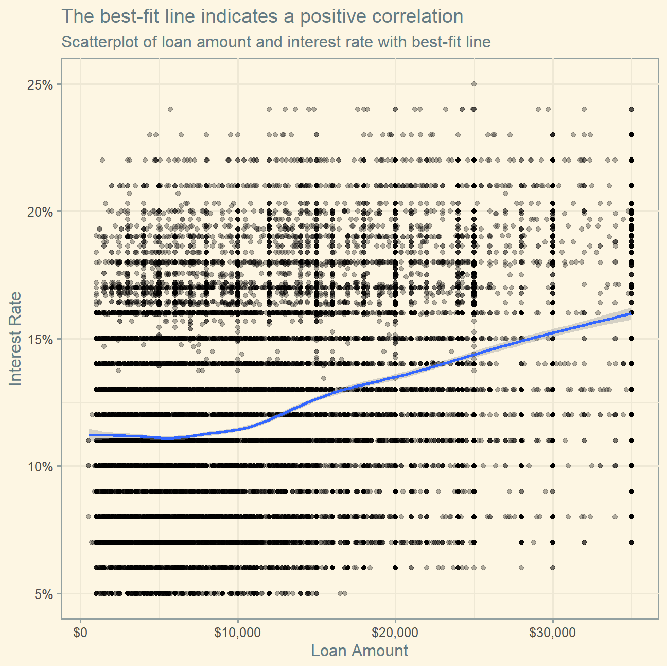

# Produce a scatter plot of annual income against interest rate and add visually the line of best fit 
lc_clean %>% 
  ggplot(aes(x = annual_inc, y = int_rate)) +
    geom_point(alpha = 0.3) + # reduce opacity to improve readability
    geom_smooth() +
    scale_x_log10(labels = scales::dollar) + # change income to log scale to account for large range of values
    scale_y_continuous(labels = scales::percent) + # change labels y
    labs(title = "The plot does not imply a correlation between income and interest rate",
         subtitle = "Scatterplot of annual income and interest rate with best-fit line",
         x = "Loan Amount",
         y = "Interest Rate") +
    theme_solarized()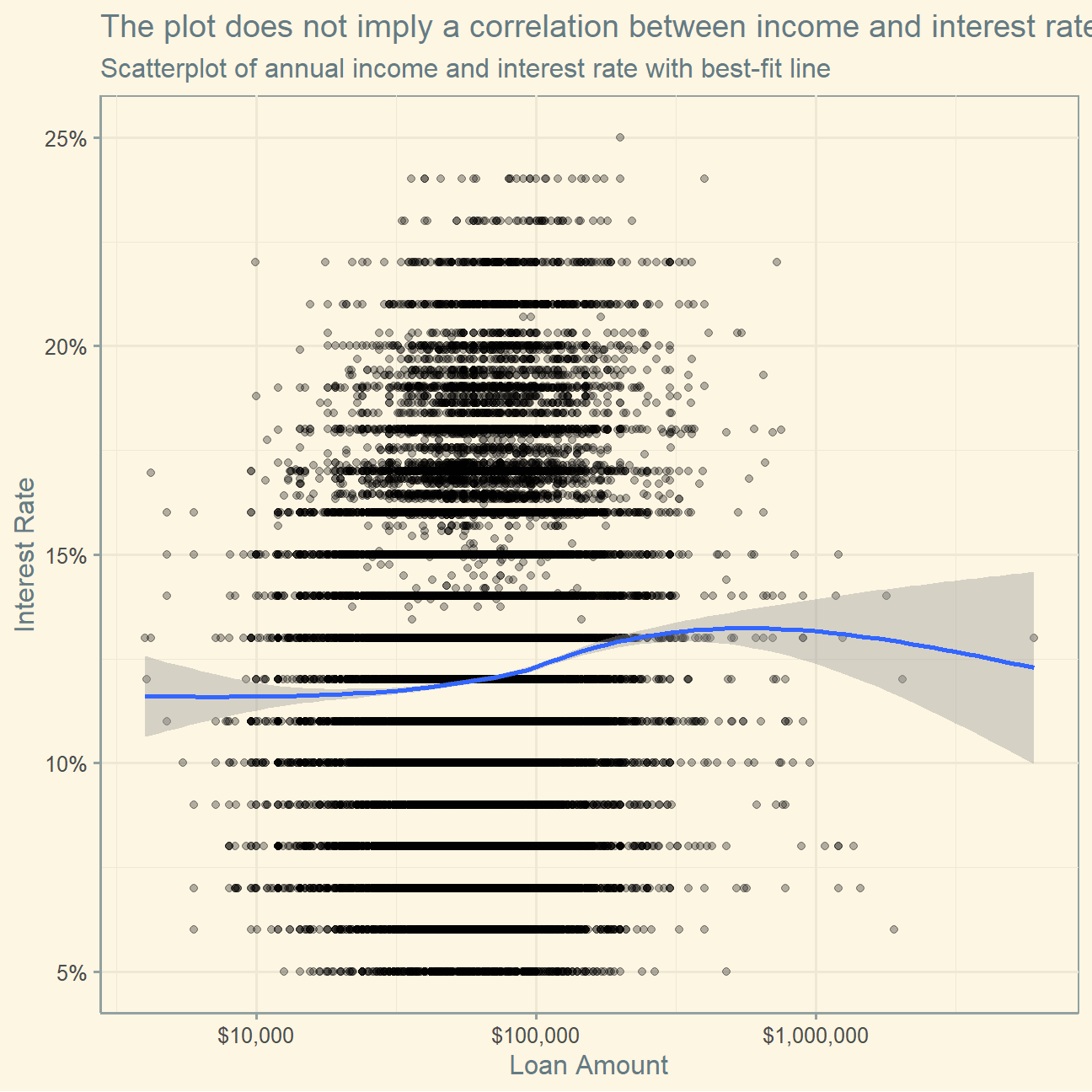

# In the same axes, produce box plots of the interest rate for every value of delinquencies
lc_clean %>% 
  ggplot(aes(x = delinq_2yrs, y = int_rate)) +
    geom_boxplot() +
    scale_y_continuous(labels = scales::percent) + # change labels y
    labs(title = "Number of delinquencies seems to affect the loan interest rate",
         subtitle = "Boxplots of interest rate by number of delinquencies in last 2 years",
         x = "Number of Delinquencies in last 2 Years",
         y = "Interest Rate") +
    theme_solarized()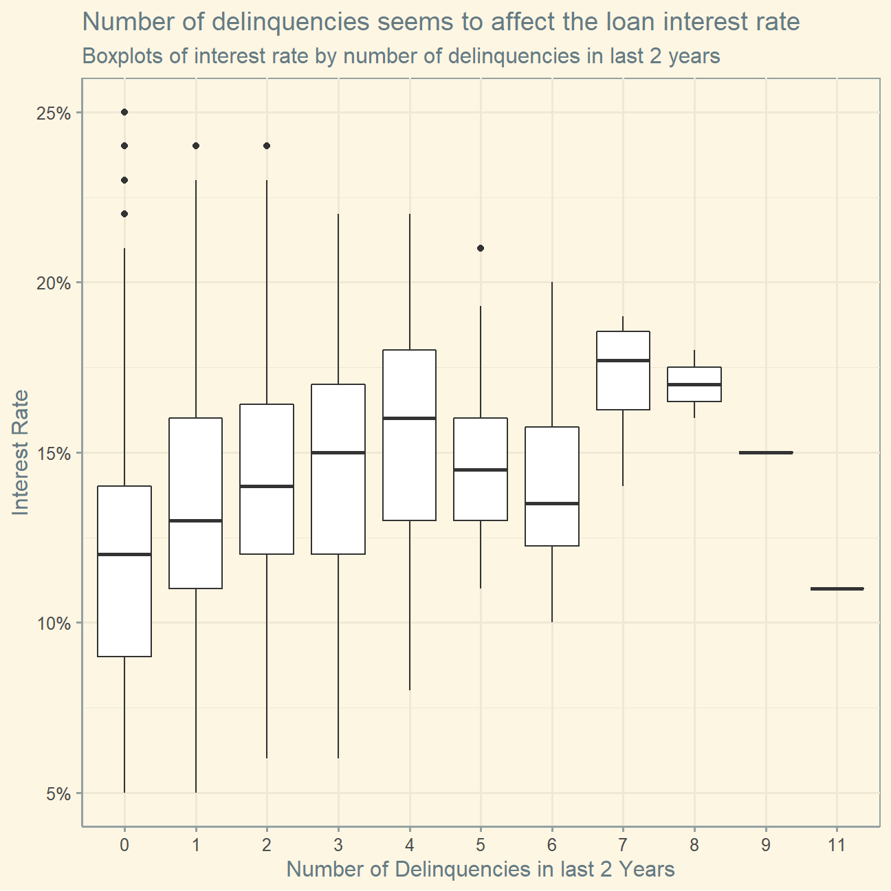

# Add 2 visualizations of your own
# Plot average dti by state in the US
int_avg_state <- lc_clean %>% 
  group_by(addr_state) %>% 
  summarize(values = mean(dti)) %>% 
  rename(state = addr_state)

  plot_usmap(data = int_avg_state, values = "values") +
    scale_fill_continuous(name = "Average DTI") +
    theme(legend.position = "right") +
    labs(title = "Central US states have higher average DTI",
         subtitle = "Average DTI per state in the US")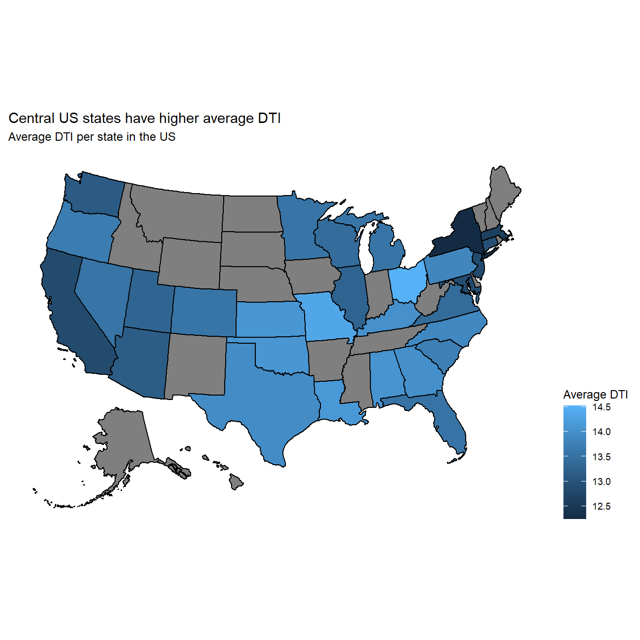

# Plot total monthly loan amount and average monthly DTI
coeff <- 1
  
lc_clean %>% 
  group_by(issue_d) %>% 
  summarize(avg_interest = mean(dti),
            sum_loan = sum(loan_amnt)/1000000) %>% 
  ggplot(aes(x = issue_d)) +
    geom_col(aes(y = sum_loan), fill = "red") +
    geom_line(aes(y = avg_interest/coeff)) +
    scale_y_continuous(name = "Total Loan Amount (in M USD)",
                     sec.axis = sec_axis(~.*coeff, name = "Average DTI")) +
    labs(x = "Time",
       title = "DTI has stayed rather stable given increasing total loan amount",
       subtitle = "Barplot of total monthly loan amount versus lineplot of average monthly DTI") +
    theme_solarized()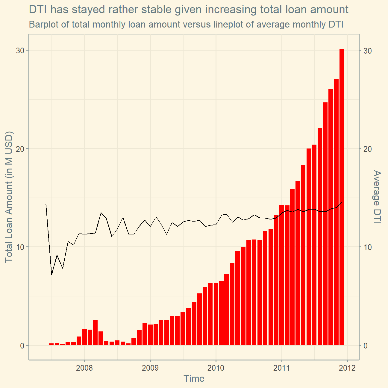

# Loan amount density faceted by grade
lc_clean %>% 
  ggplot(aes(x = loan_amnt, fill = grade)) +
    geom_density(alpha = 0.3) +
    facet_grid(grade ~ .) +
    labs(title = "Grade A to D loans display similar frequency patterns",
         subtitle = "Faceted density plot of loan amount by loan grade",
         x = "Loan Amount",
         y = "Frequency") +
    scale_x_continuous(labels = scales::dollar) +
    theme_solarized() +
    theme(legend.position = "none")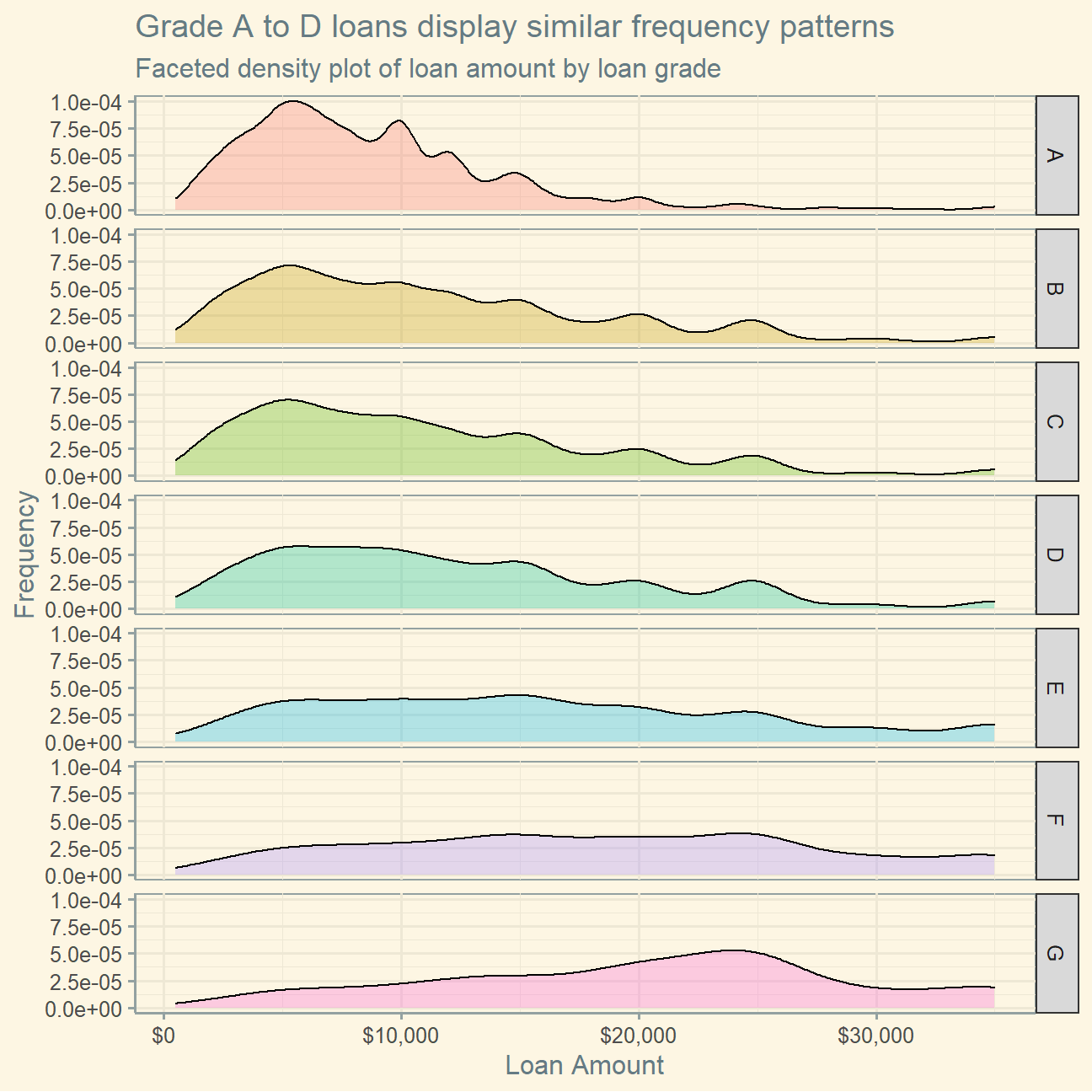

Estimate simple linear regression models

model0 <- lm(int_rate ~ term + annual_inc + dti + grade, data = lc_clean)
summary(model0)

## 
## Call:
## lm(formula = int_rate ~ term + annual_inc + dti + grade, data = lc_clean)
## 
## Residuals:
##      Min       1Q   Median       3Q      Max 
## -0.11867 -0.00745  0.00028  0.00662  0.03515 
## 
## Coefficients:
##             Estimate Std. Error t value Pr(>|t|)    
## (Intercept) 7.25e-02   1.63e-04  443.62  < 2e-16 ***
## term60      4.28e-03   1.37e-04   31.18  < 2e-16 ***
## annual_inc  3.73e-09   8.94e-10    4.18  2.9e-05 ***
## dti         5.36e-05   8.28e-06    6.47  9.7e-11 ***
## gradeB      3.58e-02   1.49e-04  239.65  < 2e-16 ***
## gradeC      6.03e-02   1.66e-04  362.75  < 2e-16 ***
## gradeD      8.20e-02   1.91e-04  429.91  < 2e-16 ***
## gradeE      1.01e-01   2.47e-04  406.44  < 2e-16 ***
## gradeF      1.20e-01   3.66e-04  328.89  < 2e-16 ***
## gradeG      1.37e-01   6.21e-04  219.99  < 2e-16 ***
## ---
## Signif. codes:  0 '***' 0.001 '**' 0.01 '*' 0.05 '.' 0.1 ' ' 1
## 
## Residual standard error: 0.0106 on 37859 degrees of freedom
## Multiple R-squared:  0.919,  Adjusted R-squared:  0.919 
## F-statistic: 4.78e+04 on 9 and 37859 DF,  p-value: <2e-16

Are all variables statistically significant?
How much explanatory power does the model have?

To gauge the statistical significance of the variables, we can look both at the t- and p-value. As the regression is based on a confidence level of 95%, we consider any t-value above roughly 2 to indicate significance. Equally, if the p-value is smaller than the significance level (here 0.05), we can claim that the variable is significant. The regression table above clearly shows that all the variables fulfill both of these criteria. The level of significance is further hinted by the star rating provided.

The adjusted R-squared is around 0.92, which is rather high. This means that 92% of the variability in interest rate is explained by the listed variables.

Fit a new linear regression that is identical to model 0, however, with the extra variable “loan_amnt”.

model1 <-lm(int_rate ~ term + annual_inc + dti + grade + loan_amnt, data = lc_clean)
summary(model1)

## 
## Call:
## lm(formula = int_rate ~ term + annual_inc + dti + grade + loan_amnt, 
##     data = lc_clean)
## 
## Residuals:
##      Min       1Q   Median       3Q      Max 
## -0.11883 -0.00704 -0.00034  0.00683  0.03508 
## 
## Coefficients:
##              Estimate Std. Error t value Pr(>|t|)    
## (Intercept)  7.17e-02   1.69e-04  424.36  < 2e-16 ***
## term60       3.61e-03   1.42e-04   25.43  < 2e-16 ***
## annual_inc  -9.73e-10   9.28e-10   -1.05     0.29    
## dti          4.33e-05   8.27e-06    5.23  1.7e-07 ***
## gradeB       3.55e-02   1.49e-04  238.25  < 2e-16 ***
## gradeC       6.02e-02   1.66e-04  362.78  < 2e-16 ***
## gradeD       8.17e-02   1.91e-04  428.75  < 2e-16 ***
## gradeE       1.00e-01   2.48e-04  402.66  < 2e-16 ***
## gradeF       1.20e-01   3.67e-04  325.41  < 2e-16 ***
## gradeG       1.35e-01   6.21e-04  218.24  < 2e-16 ***
## loan_amnt    1.48e-07   8.28e-09   17.81  < 2e-16 ***
## ---
## Signif. codes:  0 '***' 0.001 '**' 0.01 '*' 0.05 '.' 0.1 ' ' 1
## 
## Residual standard error: 0.0106 on 37858 degrees of freedom
## Multiple R-squared:  0.92,   Adjusted R-squared:  0.92 
## F-statistic: 4.34e+04 on 10 and 37858 DF,  p-value: <2e-16

Are all variables statistically significant?
If your answer to part ‘a’ is affirmative, then discuss whether model 0 should be preferred over model 1. Otherwise, discuss how a variable that was statistically significant in model 0 is not significant anymore; or how the new variable is not statistically significant.
How do you interpret the coefficients of the (i) “term60” dummy variable; (ii) “gradeF” dummy variable; and (iii) “loan_amnt” variable?
How much explanatory power does the model have?
Approximately, how wide would the 95% confidence interval of any prediction based on this model be?

All variables expect for annual income, which has a low absolute t-value of 1.049 and a high p-value of 0.294, are significant.

The reason that annual_inc is no longer statistically significant (as seen in answer a) is beause the variability in the data that was previously explained by annual_inc is now explained by loan_amnt.

All other things being equal, interest rate increases by 0.003608 when the term of the loan is 60 months as compared to 36 months All other things being equal, interest rate increases by 0.1195 when the grade of the loan is F as compared to a loan with grade A All other things being equal, interest rate increases by 0.0000001475 for every dollar increase in the loan amount

The adjusted R-squared is around 0.92, which means that 92% of the variability in the data is explained by the model. This is quite a high value and similar to model 0.

Margin of Error = 0.01056 * 2 = 0.02112, the width of 95% confidence interval should be around 2 * Margin of Error = 0.04224

Feature Engineering

Let’s build progressively more complex models, with more features.

#Add to model 1 an interaction between loan amount and grade. Use the "var1*var2" notation to define an interaction term in the linear regression model. This will add the interaction and the individual variables to the model. 

model2 <- lm(int_rate ~ term + annual_inc + dti + grade + loan_amnt + grade*loan_amnt, data = lc_clean)

#Add to the model you just created above the square and the cube of annual income. Use the poly(var_name,3) command as a variable in the linear regression model.  

model3 <- lm(int_rate ~ term + annual_inc + dti + grade + loan_amnt + grade*loan_amnt + poly(annual_inc,2) + poly(annual_inc,3), data = lc_clean)

#Continuing with the previous model, instead of annual income as a continuous variable break it down into quartiles and use quartile dummy variables. This is an alternative way of modelling non-linear relationships. You can do this with the following command. 
  
lc_clean <- lc_clean %>% 
  mutate(quartiles_annual_inc = as.factor(ntile(annual_inc, 4)))

model4 <- lm(int_rate ~ term + quartiles_annual_inc + dti + grade + loan_amnt + grade*loan_amnt, data = lc_clean)

#Compare the performance of these four models using the `anova` command
anova(model1, model2, model3, model4)

Res.Df	RSS	Df	Sum of Sq	F	Pr(>F)
3.79e+04	4.22
3.79e+04	4.19	6	0.0332	50	1.64e-61
3.78e+04	4.19	2	0.000107	0.484	0.616
3.78e+04	4.19	0	0.000915

Which of the four models has the most explanatory power in sample? Without testing on a test set, which model would you say has the highest out of sample explanatory power?
In model 2, how do you interpret the estimated coefficient of the interaction term between grade C and loan amount?
The problem of multicollinearity describes the situations where one feature is highly correlated with other features (or with a linear combination of other features). If your goal is to use the model to make predictions, should you be concerned by the problem of multicollinearity? Why, or why not?

Models 2 to 4 have exactly the same R-squared and model 1’s R-squared is very close. Therefore, the explanatory power of the models based on the R-squared is equal. Model 2 will have the highest out of sample explanatory power since the p-value for F-test is the lowest and significant for this model. This mean that the model tends to have low variance should perform well on out of sample data sets.

The coefficient indicates how an increase of one unit in loan amount differently affects a grade C loan compared to a grade A loan. The variable loan_amnt tells us that for every unit increase in loan_amnt, interest rate will rise by 0.0000001528, regardless of grade. If we then look at the interaction variable, a grade C loan will additionally decrease by 0.0000001704 for every unit increase in loan_amnt.

Multicollinearity will only affet predictive performance of the model if the covariance between variables in the training and test dataset is different. Since our sample consists of random observations in the population, we expect the same covariance for a test dataset and therefore no impact on predictive performance.

Out of sample testing

# split the data in dataframe called "testing" and another one called  "training". The "training" dataframe should have 80% of the data and the "testing" dataframe 20%.
set.seed(23)
train_test_split <- initial_split(lc_clean, prop = 0.80)
training <- training(train_test_split)
testing <- testing(train_test_split)

#Fit model2 on the training set 
model2_training<-lm(int_rate ~ term + annual_inc + dti + grade + loan_amnt + grade*loan_amnt, data = training)

# Calculate the RMSE of the model in the training set (in sample)
rmse_training<-  # take the residuals
  sqrt(mean(residuals(model2)^2))
# Use the model to make predictions out of sample in the testing set
pred<-predict(model2_training,testing)
# Calculate the RMSE of the model in the testing set (out of sample)
rmse_testing<- RMSE(pred,testing$int_rate)

cat("in-sample rmse",rmse_training)

## in-sample rmse 0.0105

cat("\nout-of-sample rmse",rmse_testing)

## 
## out-of-sample rmse 0.0106

cat("\npercentage change in error",(rmse_testing - rmse_training)/rmse_training*100,"%")

## 
## percentage change in error 0.886 %

The prediction accuracy for out-of-sample is only 1% higher than the in-sample one for seed 23, which means the model has low variance, no overfitting is detected. The result is not very sensitive to the random seed chosen. If for example we use seed 1234, we get a percentage change in error of around 2.3%, which is still a very small deterioration. For some seeds, like 784, we can even see a negative change in error between the train and test data.

k-fold cross validation

We can also do out of sample testing using the method of k-fold cross validation which has several advantages over the traditional hold-out method. Using the caret package this is easy.

#the method "cv" stands for cross validation. We re going to create 10 folds.  

control <- trainControl (
    method="cv",
    number=10,
    verboseIter=FALSE) #by setting this to true the model will report its progress after each estimation

#we are going to train the model and report the results using k-fold cross validation

plsFit10<-train(
    int_rate ~ loan_amnt + term+ dti + annual_inc + grade +grade:loan_amnt ,
    lc_clean,
   method = "lm",
    trControl = control
   )
  
cat("10-fold RMSE",plsFit10$results$RMSE)

## 10-fold RMSE 0.0105

# 5-fold
control5 <- trainControl (
    method="cv",
    number=5,
    verboseIter=FALSE) #by setting this to true the model will report its progress after each estimation

#we are going to train the model and report the results using k-fold cross validation

plsFit5<-train(
    int_rate ~ loan_amnt + term+ dti + annual_inc + grade +grade:loan_amnt ,
    lc_clean,
   method = "lm",
    trControl = control5
   )

cat("\n5-fold RMSE",plsFit5$results$RMSE)

## 
## 5-fold RMSE 0.0105

# 15-fold
control15 <- trainControl (
    method="cv",
    number=15,
    verboseIter=FALSE) #by setting this to true the model will report its progress after each estimation

#we are going to train the model and report the results using k-fold cross validation

plsFit15<-train(
    int_rate ~ loan_amnt + term+ dti + annual_inc + grade +grade:loan_amnt ,
    lc_clean,
   method = "lm",
    trControl = control15
   )

cat("\n15-fold RMSE",plsFit15$results$RMSE)

## 
## 15-fold RMSE 0.0105

The out-of-sample RMSE is a ever so slightly lower for 10-fold cross validation when compared to the hold-out method with seed 23. In general, 10-fold cross validation is more reliable since it is trained on multiple train-test splits and uses every data point for training and testing. Nevertheless, the hold-out method is still applicable if the data set is large enough. A significant drawback of k-fold cross validation is that it needs more computational power than the hold-out method, especially when folds are increased and we are working with a lot of predictors. Typically the more folds we have, the lower our out-of-sample RMSE. However, we can see that the RMSE change only very minutely between number of folds, meaning that our model is very robust.

Sample size estimation and learning curves

We can use the hold out method for out-of-sample testing to check if we have a sufficiently large sample to estimate the model reliably. The idea is to set aside some of the data as a testing set. From the remaining data draw progressively larger training sets and check how the performance of the model on the testing set changes. If the performance no longer improves with larger training sets we know we have a large enough sample. The code below does this. Examine it and run it with different random seeds.

# select a testing dataset (25% of all data)
set.seed(1234)

train_test_split <- initial_split(lc_clean, prop = 0.75)
remaining <- training(train_test_split)
testing <- testing(train_test_split)

# We are now going to run 30 models starting from a tiny training set drawn from the training data and progressively increasing its size. The testing set remains the same in all iterations.

#initiating the model by setting some parameters to zero
rmse_sample<-0
sample_size<-0
Rsq_sample<-0

for(i in 1:30) {
#from the remaining dataset select a smaller subset to training the data
set.seed(1234)
sample

  learning_split <- initial_split(remaining, prop = i/100)
  training <- training(learning_split)
  sample_size[i]=nrow(training)
  
  # training the model on the small dataset
  model3<-lm(int_rate ~ loan_amnt + term+ dti + annual_inc + grade + grade:loan_amnt, training)
  # test the performance of the model on the large testing dataset. This stays fixed for all iterations.
  pred<-predict(model3,testing)
  rmse_sample[i]<-RMSE(pred,testing$int_rate)
  Rsq_sample[i]<-R2(pred,testing$int_rate)
}
plot(sample_size,rmse_sample)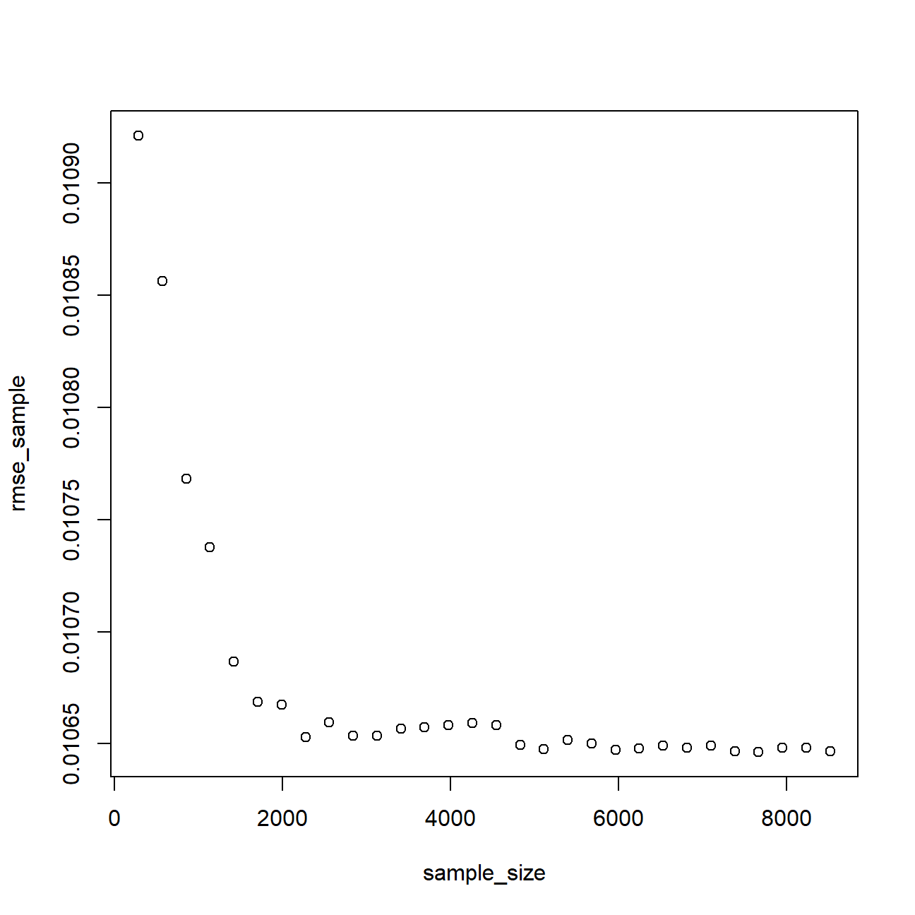

plot(sample_size,Rsq_sample)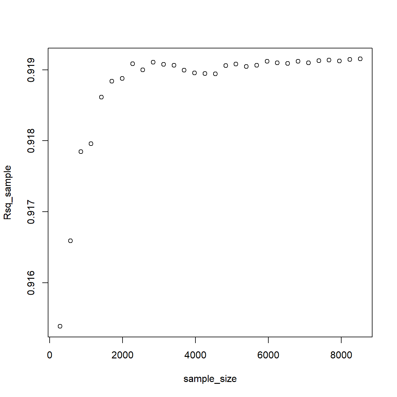

A sample of a little less than 6000 observations would be enough to estimate model 3 reliably. We can see that at that stage, the points on the RMSE and R-squared flatten out and start to fluctuate, so an increase in sample size is no longer beneficial. We have several ways to reduce prediction error further after reaching a critical sample size, including automated feature selection to identify the right features or implement Lasso to reduce irrelevant variables.

Regularization using LASSO regression

#split the data in testing and training. The training test is really small.

set.seed(1234)
train_test_split <- initial_split(lc_clean, prop = 0.01)
training <- training(train_test_split)
testing <- testing(train_test_split)

model_lm<-lm(int_rate ~ poly(loan_amnt,3) + term + dti + annual_inc + grade + grade:poly(loan_amnt,3):term + poly(loan_amnt,3):term + grade:term, training)
predictions <- predict(model_lm,testing)

# Model prediction performance

data.frame(
  RMSE = RMSE(predictions, testing$int_rate),
  Rsquare = R2(predictions, testing$int_rate)
)

RMSE	Rsquare
0.0123	0.891

Not surprisingly this model does not perform well – as we knew form the learning curves we constructed for a simpler model we need a lot more data to estimate this model reliably. Try running it again with different seeds. The model’s performance tends to be sensitive to the choice of the training set.

LASSO regression offers one solution – it extends the OLS regression by penalizing the model for setting any coefficient estimate to a value that is different from zero. The penalty is proportional to a parameter \(\lambda\) (pronounced lambda). This parameter cannot be estimated directly (and for this reason sometimes it is referred to as hyperparameter). \(\lambda\) will be selected through k-fold cross validation so as to provide the best out-of-sample performance. As a result of the LASSO procedure, only those features that are more strongly associated with the outcome will have non-zero coefficient estimates and the estimated model will be less sensitive to the training set. Sometimes LASSO regression is referred to as regularization.

set.seed(1234)
# we will look for the optimal lambda in this sequence (we will try 1000 different lambdas, feel free to try more if necessary)
lambda_seq <- seq(0, 0.01, length = 1000)

# lasso regression using k-fold cross validation to select the best lambda

lasso <- train(
 int_rate ~ poly(loan_amnt,3) + term+ dti + annual_inc + grade +grade:poly(loan_amnt,3):term +poly(loan_amnt,3):term +grade:term,
 data = training,
 method = "glmnet",
  preProc = c("center", "scale"), #This option standardizes the data before running the LASSO regression
  trControl = control,
  tuneGrid = expand.grid(alpha = 1, lambda = lambda_seq) #alpha=1 specifies to run a LASSO regression.
  )

# Model coefficients
coef(lasso$finalModel, lasso$bestTune$lambda)

## 58 x 1 sparse Matrix of class "dgCMatrix"
##                                          s1
## (Intercept)                        1.21e-01
## poly(loan_amnt, 3)1                7.80e-04
## poly(loan_amnt, 3)2                .       
## poly(loan_amnt, 3)3                .       
## term60                             1.40e-03
## dti                                3.87e-04
## annual_inc                         .       
## gradeB                             1.65e-02
## gradeC                             2.30e-02
## gradeD                             2.47e-02
## gradeE                             2.47e-02
## gradeF                             1.88e-02
## gradeG                             1.74e-02
## poly(loan_amnt, 3)1:term60         .       
## poly(loan_amnt, 3)2:term60         .       
## poly(loan_amnt, 3)3:term60         .       
## term60:gradeB                     -7.87e-04
## term60:gradeC                      .       
## term60:gradeD                      4.70e-04
## term60:gradeE                      1.67e-03
## term60:gradeF                      6.39e-04
## term60:gradeG                      1.50e-03
## poly(loan_amnt, 3)1:term36:gradeB  .       
## poly(loan_amnt, 3)2:term36:gradeB  .       
## poly(loan_amnt, 3)3:term36:gradeB  4.36e-04
## poly(loan_amnt, 3)1:term60:gradeB  .       
## poly(loan_amnt, 3)2:term60:gradeB  3.90e-04
## poly(loan_amnt, 3)3:term60:gradeB  .       
## poly(loan_amnt, 3)1:term36:gradeC  .       
## poly(loan_amnt, 3)2:term36:gradeC  2.68e-04
## poly(loan_amnt, 3)3:term36:gradeC -7.36e-05
## poly(loan_amnt, 3)1:term60:gradeC  .       
## poly(loan_amnt, 3)2:term60:gradeC  .       
## poly(loan_amnt, 3)3:term60:gradeC -2.02e-04
## poly(loan_amnt, 3)1:term36:gradeD  .       
## poly(loan_amnt, 3)2:term36:gradeD  5.14e-04
## poly(loan_amnt, 3)3:term36:gradeD  3.15e-04
## poly(loan_amnt, 3)1:term60:gradeD  .       
## poly(loan_amnt, 3)2:term60:gradeD  .       
## poly(loan_amnt, 3)3:term60:gradeD  .       
## poly(loan_amnt, 3)1:term36:gradeE  .       
## poly(loan_amnt, 3)2:term36:gradeE  .       
## poly(loan_amnt, 3)3:term36:gradeE  .       
## poly(loan_amnt, 3)1:term60:gradeE  .       
## poly(loan_amnt, 3)2:term60:gradeE  .       
## poly(loan_amnt, 3)3:term60:gradeE -3.37e-04
## poly(loan_amnt, 3)1:term36:gradeF  .       
## poly(loan_amnt, 3)2:term36:gradeF  .       
## poly(loan_amnt, 3)3:term36:gradeF  .       
## poly(loan_amnt, 3)1:term60:gradeF  .       
## poly(loan_amnt, 3)2:term60:gradeF  .       
## poly(loan_amnt, 3)3:term60:gradeF  1.40e-03
## poly(loan_amnt, 3)1:term36:gradeG  .       
## poly(loan_amnt, 3)2:term36:gradeG  .       
## poly(loan_amnt, 3)3:term36:gradeG  .       
## poly(loan_amnt, 3)1:term60:gradeG  .       
## poly(loan_amnt, 3)2:term60:gradeG  3.88e-04
## poly(loan_amnt, 3)3:term60:gradeG  .

# Best lambda
lasso$bestTune$lambda

## [1] 0.00041

# Count of how many coefficients are greater than zero and how many are equal to zero

sum(coef(lasso$finalModel, lasso$bestTune$lambda)!=0)

## [1] 25

sum(coef(lasso$finalModel, lasso$bestTune$lambda)==0)

## [1] 33

# Make predictions
predictions <- predict(lasso,testing)

# Model prediction performance

data.frame(
  RMSE = RMSE(predictions, testing$int_rate),
  Rsquare = R2(predictions, testing$int_rate)
)

RMSE	Rsquare
0.0108	0.918

Which model performs best out of sample, OLS regression or LASSO? Why?
What value of lambda offers best performance? Is this sensitive to the random seed? Why?
How many coefficients are zero and how many are non-zero in the LASSO model of best fit? Is number of zero (or non-zero) coefficients sensitive on the random seed? Why?
Why is it important to standardize continuous variables before running LASSO?

Lasso outperforms the hold-out method for the data set, given that the RMSE for the given seed is lower and the R-squared is higher.

By setting the seed to 1234, the best value of lambda that we get is 0.0002902903 which produces RMSE equals to 0.01081854 and R-square equal to 0.9167534. By testing across different testing values of lambda (up to 5000), we’ve observed trivial changes in lambda, RMSE and R-squared. Therefore, 0.0002902903 is roughly the best lambda we can achieve. Lambda is not sensitive to the seeds because each time you run a cross validation you get an estimate of the true population test error. Different random seeds give you different estimates of the population quantity, but each is an estimate of the same underlying truth.

The Lasso model produces 30 non-zero coefficients and 28 zero coefficients at seed 1234. The number of zero coefficients barely changes when we change setting seeds; therefore, coefficient is not very sensitive to changing seeds due to the same reason mentioned in part b.

It is important to standardize continuous variables because they are often measured in different units. As Lasso limits the coefficients of each variable, the magnitude has to be made comparable between variables, which is only possible through standardization.

set.seed(1234)
# we will look for the optimal lambda in this sequence (we will try 1000 different lambdas, feel free to try more if necessary)
lambda_seq <- seq(0, 0.01, length = 1000)

# ridge regression using k-fold cross validation to select the best lambda

ridge <- train(
 int_rate ~ poly(loan_amnt,3) + term+ dti + annual_inc + grade +grade:poly(loan_amnt,3):term +poly(loan_amnt,3):term +grade:term,
 data = training,
 method = "glmnet",
  preProc = c("center", "scale"), #This option standardizes the data before running the Ridge regression
  trControl = control,
  tuneGrid = expand.grid(alpha = 0, lambda = lambda_seq) #alpha=0 specifies to run a Ridge regression.
  )

# Make predictions
predictions_ridge <- predict(ridge,testing)

# Model prediction performance

data.frame(
  RMSE = RMSE(predictions_ridge, testing$int_rate),
  Rsquare = R2(predictions_ridge, testing$int_rate)
)

RMSE	Rsquare
0.0214	0.694

Which model performs best out of sample, OLS regression, LASSO, or Ridge?
What value of lambda offers best performance?
How many coefficients are zero and how many are non-zero in the Ridge model of best fit? How does it compare with the LASSO regression and what is the reason of the difference?
Is it important to standardize continuous variables before running Ridge as in LASSO? Or is it less important for the Ridge regression?
In class, we studied the advantages of LASSO regression over the standard OLS. Discuss one potential advantage of using the Ridge regression over the OLS.

Given the same seed of 1234, LASSO still performs better than both OLS and Ridge, as the R-squared is the highest and RMSE the lowest among the three.

At seed 1234, the best performing lamba has a value of 0.0002902903 for the LASSO regression. It has to be mentioned that the best performing lambda for Ridge is higher at 0.001601602 at seed 1234.

All 58 variables in the Ridge regression have a coefficient that is non-zero, whereas the LASSO regression has 28 variables with a coefficient of 0.The reason we see a difference is that Ridge minimizs the coefficients, but never sets them to absolute 0.

It is just as important to standardize values in the ridge regression as compared to LASSO, as it also tries to limit values based on lambda.

Ridge regression is advantageous over OLS in its ability to deal with variables that are highly collinear. Instead of having to identify and eliminate colinear predictors step by step in OLS, Ridge addresses colinearity in its calculation. Where LASSO regression randomly picks one of the colinear variables and excludes the others, Ridge will keep all variables and still account for the multicolinearity.

Using Time Information

set.seed(1234)
#linear time trend -- concentrate on the interest rate as a function of the time (add code below)
linear_time_trend <-lc_clean %>%
  select(int_rate, issue_d) %>%
  group_by(issue_d) %>%
  summarise(int_rate_mean = mean(int_rate, na.rm = TRUE)) %>%
  ggplot(aes(issue_d, int_rate_mean)) +
    geom_line(color= "darkblue", size = 1) +
    labs(x = "Time", 
         y = "Average Interest Rate", 
         title = "The average interest rate has been increasing since 2007",
         subtitle = "Lineplot of average interest rate over time") +
    scale_y_continuous(labels = scales::percent) + # change labels y
    theme_solarized()

linear_time_trend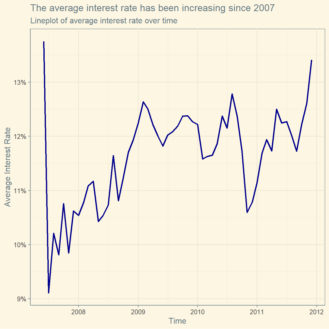

#linear time trend by grade -- similar plot, however, group by grades (via different colors) (add code below)
linear_time_trend_by_grade <-lc_clean %>%
  select(int_rate, issue_d, grade) %>%
  group_by(issue_d, grade) %>%
  summarise(int_rate_mean = mean(int_rate, na.rm = TRUE)) %>%
  ggplot(aes(issue_d, int_rate_mean, color = grade, group = grade)) +
    geom_line()+
    labs(x = "Time", 
         y = "Average Interest Rate", 
         title = "The average interest rate has followed a similar pattern across all grades",
         subtitle = "Faceted lineplot of average interest rate over time by grade",
         color = "Grade") +
    scale_y_continuous(labels = scales::percent) + # change labels y
    theme_solarized()

linear_time_trend_by_grade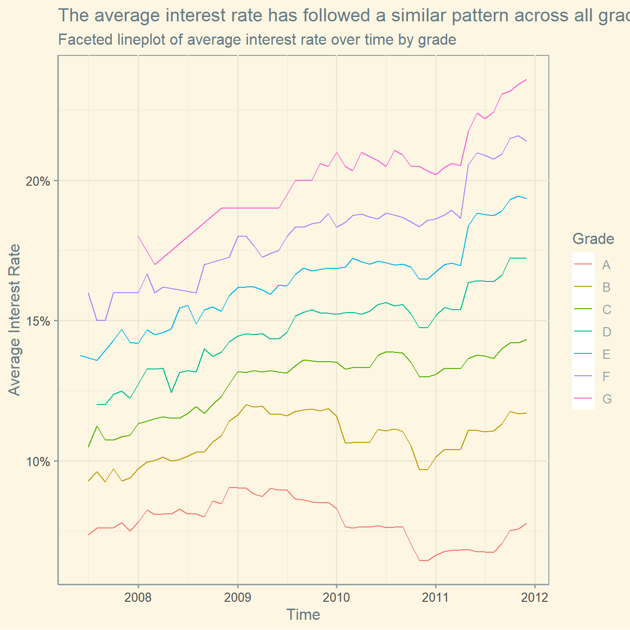

#Train models using OLS regression and k-fold cross-validation
#The first model has some explanatory variables and a linear time trend

time1<-train(
  int_rate ~ issue_d + grade + term + annual_inc + dti  + loan_amnt,
  lc_clean,
  method = "lm",
  trControl = control)

#The second model has a different linear time trend for each grade class (hint. use interactions)
time2<-train(
    int_rate ~ issue_d * grade + term + annual_inc + dti + loan_amnt,
    lc_clean,
   method = "lm",
    trControl = control
   )

#Change the time trend to a quarter dummy variables.
#zoo::as.yearqrt() creates quarter dummies 
lc_clean_quarter<-lc_clean %>%
  mutate(yq = as.factor(as.yearqtr(lc_clean$issue_d, format = "%Y-%m-%d")))

time3<-train(
    int_rate ~ yq + grade + term + annual_inc + dti + loan_amnt,
    lc_clean_quarter,
     method = "lm",
    trControl = control
   )

#We specify one quarter dummy variable for each grade. This is going to be a large model as there are 19 quarters x 7 grades = 133 quarter-grade dummies.
time4<-train(
    int_rate ~ yq * grade + term + annual_inc + dti + loan_amnt,
    lc_clean_quarter,
     method = "lm",
    trControl = control
   )

data.frame(
  time1$results$RMSE,
  time2$results$RMSE,
  time3$results$RMSE,
  time4$results$RMSE)

time1.results.RMSE	time2.results.RMSE	time3.results.RMSE	time4.results.RMSE
0.0104	0.00907	0.00913	0.00762

According to the graphs above, we can observe distinct interest fluctuation over time and constant patterns across grades. Therefore, we would infer that interest rates change over time according to the graphs. Including quarter-year dummies improved the predictive performance of the models. When looking at the RMSEs in the table above, we can observe that quarter dummy variables and an interaction term between grade and time reduced the RMSE of the model from around 0.01 to roughly 0.009. Escpecially an interaction term between quarter and grade stood out as effective, with an RMSE of around 0.0076. This is not surprising, as quarters should be more representative of fluctuations in the general economy, which we expect to be behind the fluctations of interest rate over time. Still, we cannot use time as a variable to predict future interest rates, only past ones.

Using Bond Yields

#load the data to memory as a dataframe
bond_prices<-readr::read_csv("data/MonthBondYields .csv")

#make the date of the bond file comparable to the lending club dataset
#for some regional date/number (locale) settings this may not work. If it does try running the following line of code in the Console
Sys.setlocale("LC_TIME","English")

## [1] "English_United States.1252"

bond_prices <- bond_prices %>%
  mutate(Date2=as.Date(paste("01",Date,sep="-"),"%d-%b-%y")) %>%
  select(-starts_with("X"))

#let's see what happened to bond yields over time. Lower bond yields mean the cost of borrowing has gone down.

bond_prices %>%
  ggplot(aes(x=Date2, y=Price))+
  geom_point(size=1, alpha=0.5, color = "red") +
  labs(title = "Bond yields are gradually increasing between 2007 and 2012",
         subtitle = "Scatterplot of bond price over time",
         x = "Time",
         y = "Bond Price") +
    scale_y_continuous(labels = scales::dollar_format()) + # change labels
    theme_solarized()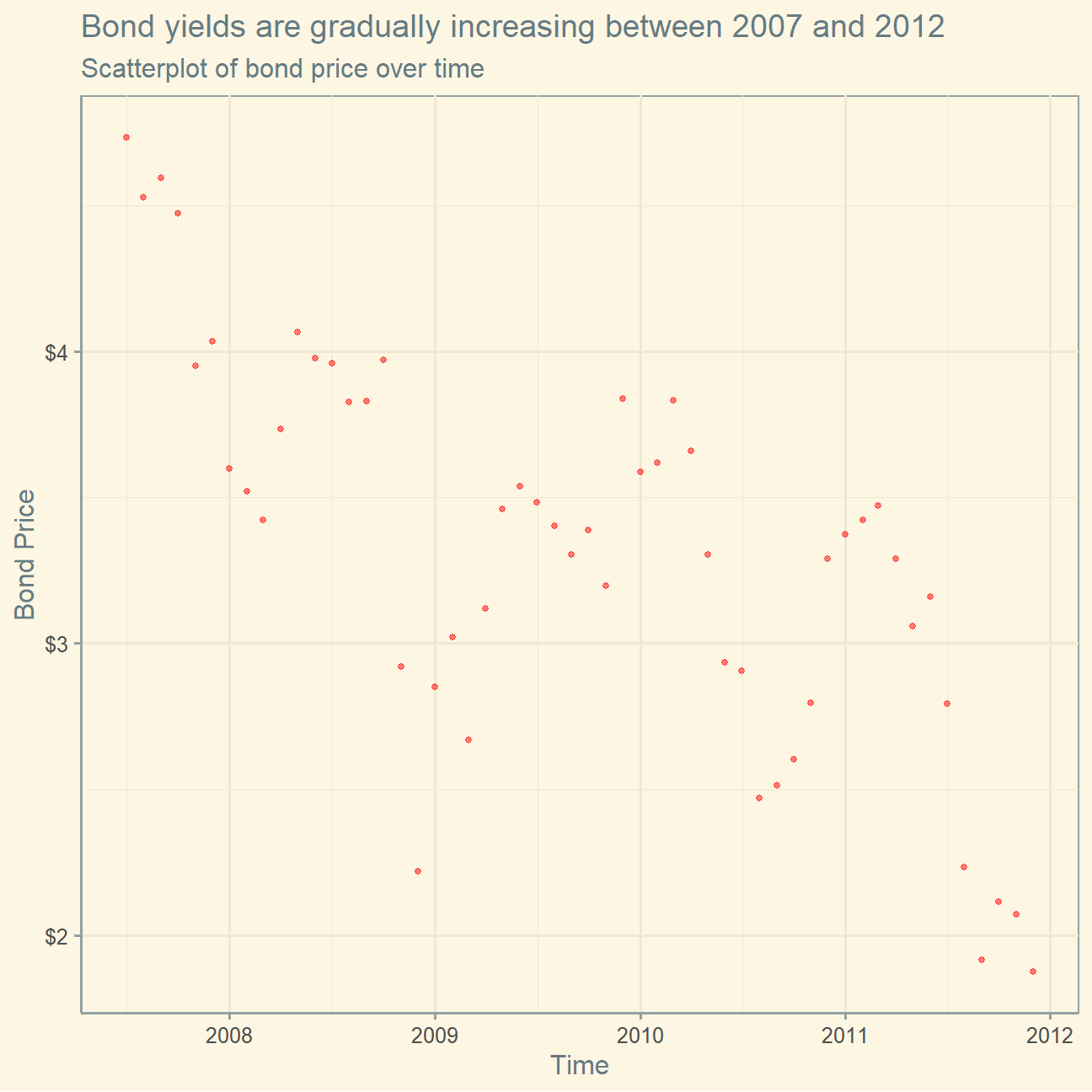

#join the data using a left join
lc_with_bonds<-lc_clean %>%
  left_join(bond_prices, by = c("issue_d" = "Date2")) %>%
  arrange(issue_d) %>%
  filter(!is.na(Price)) #drop any observations where there re no bond prices available

# investigate graphically if there is a relationship 
lc_with_bonds%>%
  ggplot(aes(x=int_rate, y=Price))+
  geom_point(size=0.8, alpha=0.5, color = "red")+
  geom_smooth(method="lm") +
  labs(title = "Interest rate increases as bond yields rise",
         subtitle = "Scatterplot of interest rate and bond price with best-fit line",
         x = "Interest Rate",
         y = "Bond Price") +
    scale_x_continuous(labels = scales::percent) + # change labels
    scale_y_continuous(labels = scales::dollar) + # change labels
    theme_solarized()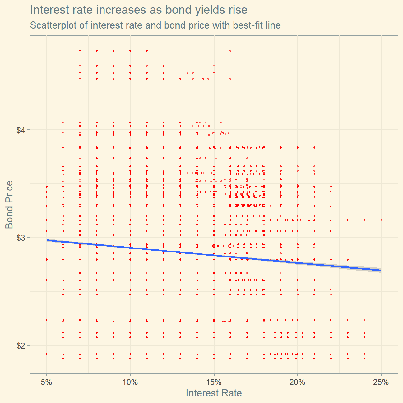

lc_with_bonds%>%
  ggplot(aes(x=int_rate, y=Price, color=grade))+
  geom_point(size=0.8, alpha=0.5)+
  geom_smooth(method="lm") +
  labs(title = "Grade A loan interest rate do not seem affected by by bond yield",
         subtitle = "Colored scatterplot of interest rate and bond price with best-fit line",
         x = "Interest Rate",
         y = "Bond Price",
         color = "Grade") +
    scale_x_continuous(labels = scales::percent) + # change labels
    scale_y_continuous(labels = scales::dollar) + # change labels
    theme_solarized()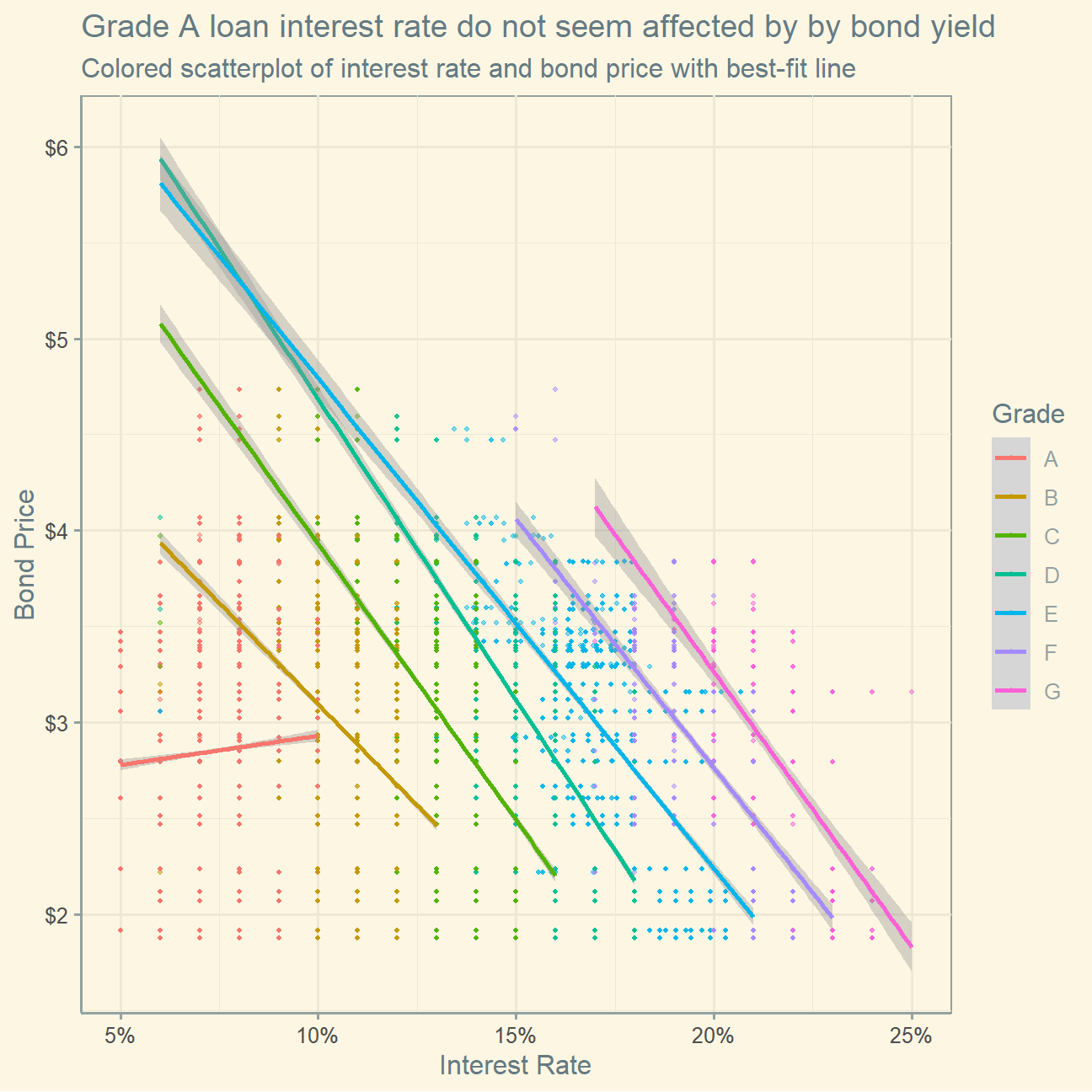

#let's train a model using the bond information

plsFit<-train(
    int_rate ~ Price + grade, #fill your variables here -- try adding Price and grade.
    lc_with_bonds,
   method = "lm",
    trControl = control #add 10-fold CV control here
   )
summary(plsFit)

## 
## Call:
## lm(formula = .outcome ~ ., data = dat)
## 
## Residuals:
##      Min       1Q   Median       3Q      Max 
## -0.11886 -0.00649 -0.00005  0.00674  0.03802 
## 
## Coefficients:
##              Estimate Std. Error t value Pr(>|t|)    
## (Intercept)  8.99e-02   2.65e-04   338.7   <2e-16 ***
## Price       -5.72e-03   8.57e-05   -66.8   <2e-16 ***
## gradeB       3.68e-02   1.41e-04   261.5   <2e-16 ***
## gradeC       6.19e-02   1.56e-04   397.8   <2e-16 ***
## gradeD       8.38e-02   1.76e-04   475.2   <2e-16 ***
## gradeE       1.03e-01   2.21e-04   468.5   <2e-16 ***
## gradeF       1.24e-01   3.36e-04   368.1   <2e-16 ***
## gradeG       1.40e-01   5.86e-04   239.4   <2e-16 ***
## ---
## Signif. codes:  0 '***' 0.001 '**' 0.01 '*' 0.05 '.' 0.1 ' ' 1
## 
## Residual standard error: 0.0102 on 37860 degrees of freedom
## Multiple R-squared:  0.926,  Adjusted R-squared:  0.926 
## F-statistic: 6.73e+04 on 7 and 37860 DF,  p-value: <2e-16

Bond yields have strong explanatory powers. Typically the lower the higher the bond yield, the higher the interest rate (Grade B to G all show this pattern), as bond price indicates the economic situation. Right now the UK and many other developed countries are seeing a strong growth in bond yields, caused in part by rising inflation. We can assume that the increase in interest rate has to do with the opportunity cost of banks not buying bonds, so the missed bond yields are added to their interest rate. Meanwhile, the colored scatterplot of price and interest rate by grade shows that the interest rate for grade A loans is not strongly affected by bond yield. For a loan of any grade, the model shows that an one unit increase in bond price (i.e. decrease in bond yield) causes interest rate to drop by 0.005722. Since the pattern between price and interest rate varies between grade A and other grades, it would be better if we add an interaction term of grade and price.

Choose a model and describe your methodology

# Testing for a imrpvoed normal OLS model with selected features
OLS_best <- train(
    int_rate ~ Price+ term + installment + grade + poly(loan_amnt,3) +
      grade:poly(loan_amnt,3) + poly(loan_amnt,3):term +grade:term + grade:Price,
    lc_with_bonds,
   method = "lm",
    trControl = control #add 10-fold CV
   )
summary(plsFit)

## 
## Call:
## lm(formula = .outcome ~ ., data = dat)
## 
## Residuals:
##      Min       1Q   Median       3Q      Max 
## -0.11886 -0.00649 -0.00005  0.00674  0.03802 
## 
## Coefficients:
##              Estimate Std. Error t value Pr(>|t|)    
## (Intercept)  8.99e-02   2.65e-04   338.7   <2e-16 ***
## Price       -5.72e-03   8.57e-05   -66.8   <2e-16 ***
## gradeB       3.68e-02   1.41e-04   261.5   <2e-16 ***
## gradeC       6.19e-02   1.56e-04   397.8   <2e-16 ***
## gradeD       8.38e-02   1.76e-04   475.2   <2e-16 ***
## gradeE       1.03e-01   2.21e-04   468.5   <2e-16 ***
## gradeF       1.24e-01   3.36e-04   368.1   <2e-16 ***
## gradeG       1.40e-01   5.86e-04   239.4   <2e-16 ***
## ---
## Signif. codes:  0 '***' 0.001 '**' 0.01 '*' 0.05 '.' 0.1 ' ' 1
## 
## Residual standard error: 0.0102 on 37860 degrees of freedom
## Multiple R-squared:  0.926,  Adjusted R-squared:  0.926 
## F-statistic: 6.73e+04 on 7 and 37860 DF,  p-value: <2e-16

# Creating best model using lasso regression and k-fold cross validation to select the best lambda
set.seed(1234)
train_test_split <- initial_split(lc_with_bonds, prop = 0.16)
training <- training(train_test_split)
testing <- testing(train_test_split)
lambda_seq <- seq(0, 0.01, length = 1000)
lasso_best <- train(
 int_rate ~ Price+ term + installment + grade + poly(loan_amnt,3) +
      grade:poly(loan_amnt,3) + poly(loan_amnt,3):term +grade:term + grade:Price,
 data = training,
 method = "glmnet",
  preProc = c("center", "scale"),
  trControl = control,
  tuneGrid = expand.grid(alpha = 1, lambda = lambda_seq)
  )

# Best lambda
lasso_best$bestTune$lambda

## [1] 0

# Count of how many coefficients are greater than zero and how many are equal to zero

sum(coef(lasso$finalModel, lasso$bestTune$lambda)!=0)

## [1] 25

sum(coef(lasso$finalModel, lasso$bestTune$lambda)==0)

## [1] 33

# Make predictions
predictions <- predict(lasso_best,testing)

# Model prediction performance

data.frame(
  RMSE = RMSE(predictions, testing$int_rate),
  Rsquare = R2(predictions, testing$int_rate)
)

RMSE	Rsquare
0.00637	0.971

Feel free to investigate more models with different features using the methodologies covered so far. Present the model you believe predicts interest rates the best. Describe how good it is (including the length of the 95% Confidence Interval of predictions that use this model) and what features it uses. What methodology did you use to choose it? (Do not use time trends or quarter-year dummies in your model as the first cannot be extrapolated into the future reliably and the second cannot be even estimated for future quarters.)

Answer here: The best model in terms of predictive performance is a LASSO regression depicted above and cross validated using a 10 k-fold validation. By finding the optimal lambda, we determined the coefficients for the variables. The variables we included were chosen based on their performance in previous models, for example using the polynomial for loan amount and using interaction terms to account for differences in loan grades. With a R-squared of 0.97 and an RMSE of around 0.0064 for the LASSO regression, the model outperforms most models we have explored so far. As the LASSO regression is trained on a smaller training data set than the OLS, we expect it to outperform the OLS in predicting out of sample interest rates. The size of the of the training dataset was determined with the learning curve plots in Q7 of this report, which is roughly 6000 observations or 16% of the observations. The length of the confidence interval for the final model chosen is 2 times the margin of error (2* (2 * 0.006365)), which gives us a value of 0.02546.

Use other publicly available datasets to further improve performance

set.seed(1234)

library(dint)
cpi<-readr::read_csv("data/CPI.csv")
gdp<-readr::read_csv("data/GDP.csv")
unep<- readr::read_csv("data/UNEP.csv")

cpi$quarter <- paste(year(cpi$DATE),get_quarter(cpi$DATE),sep = "-")
gdp$quarter <- paste(year(gdp$DATE),get_quarter(gdp$DATE),sep = "-")
lc_with_bonds$quarters <- paste(year(lc_with_bonds$issue_d),get_quarter(lc_with_bonds$issue_d),sep = "-")

lc_with_add <- lc_with_bonds %>%
  left_join(cpi, by = c("quarters" = "quarter")) %>%
  left_join(gdp, by = c("quarters" = "quarter")) %>%
  left_join(unep, by = c("issue_d" = "DATE")) %>%
  arrange(issue_d)

plsFit<-train(
    int_rate ~ Price+ term + installment + grade + poly(loan_amnt,3) + UNRATE + CPALTT01USQ657N + GDP +
      grade:poly(loan_amnt,3) + poly(loan_amnt,3):term +grade:term + grade:Price + grade:UNRATE + grade:CPALTT01USQ657N +
      grade:GDP,
    lc_with_add,
   method = "lm",
    trControl = control #add 10-fold CV
   )
summary(plsFit)

## 
## Call:
## lm(formula = .outcome ~ ., data = dat)
## 
## Residuals:
##      Min       1Q   Median       3Q      Max 
## -0.08429 -0.00364  0.00001  0.00342  0.02969 
## 
## Coefficients:
##                               Estimate Std. Error t value Pr(>|t|)    
## (Intercept)                  -1.17e-01   4.61e-03  -25.50  < 2e-16 ***
## Price                        -3.35e-03   1.83e-04  -18.32  < 2e-16 ***
## term60                        1.33e-01   7.07e-04  188.18  < 2e-16 ***
## installment                   1.06e-03   5.20e-06  204.05  < 2e-16 ***
## gradeB                       -1.04e-01   5.45e-03  -19.00  < 2e-16 ***
## gradeC                       -1.71e-01   5.79e-03  -29.51  < 2e-16 ***
## gradeD                       -2.42e-01   6.76e-03  -35.77  < 2e-16 ***
## gradeE                       -2.28e-01   9.29e-03  -24.51  < 2e-16 ***
## gradeF                       -1.97e-01   1.64e-02  -12.05  < 2e-16 ***
## gradeG                       -1.40e-01   3.13e-02   -4.49  7.1e-06 ***
## `poly(loan_amnt, 3)1`        -4.77e+01   2.36e-01 -201.77  < 2e-16 ***
## `poly(loan_amnt, 3)2`        -1.89e-01   1.79e-02  -10.53  < 2e-16 ***
## `poly(loan_amnt, 3)3`        -5.05e-02   1.62e-02   -3.11  0.00185 ** 
## UNRATE                       -8.06e-04   7.83e-05  -10.29  < 2e-16 ***
## CPALTT01USQ657N              -1.23e-03   1.16e-04  -10.68  < 2e-16 ***
## GDP                          -1.06e-05   2.27e-07  -46.47  < 2e-16 ***
## `gradeB:poly(loan_amnt, 3)1` -2.60e+00   2.57e-02 -101.24  < 2e-16 ***
## `gradeC:poly(loan_amnt, 3)1` -4.53e+00   3.19e-02 -141.72  < 2e-16 ***
## `gradeD:poly(loan_amnt, 3)1` -6.21e+00   3.88e-02 -160.02  < 2e-16 ***
## `gradeE:poly(loan_amnt, 3)1` -7.67e+00   4.75e-02 -161.48  < 2e-16 ***
## `gradeF:poly(loan_amnt, 3)1` -9.27e+00   6.30e-02 -147.15  < 2e-16 ***
## `gradeG:poly(loan_amnt, 3)1` -1.06e+01   1.03e-01 -102.75  < 2e-16 ***
## `gradeB:poly(loan_amnt, 3)2`  1.68e-01   2.27e-02    7.40  1.4e-13 ***
## `gradeC:poly(loan_amnt, 3)2`  1.80e-01   2.41e-02    7.45  9.3e-14 ***
## `gradeD:poly(loan_amnt, 3)2` -3.17e-02   2.54e-02   -1.25  0.21211    
## `gradeE:poly(loan_amnt, 3)2` -9.93e-02   3.00e-02   -3.31  0.00094 ***
## `gradeF:poly(loan_amnt, 3)2` -1.46e-01   4.35e-02   -3.35  0.00080 ***
## `gradeG:poly(loan_amnt, 3)2` -4.12e-02   8.38e-02   -0.49  0.62299    
## `gradeB:poly(loan_amnt, 3)3`  3.27e-03   2.05e-02    0.16  0.87313    
## `gradeC:poly(loan_amnt, 3)3` -4.22e-02   2.19e-02   -1.93  0.05415 .  
## `gradeD:poly(loan_amnt, 3)3` -1.02e-01   2.34e-02   -4.38  1.2e-05 ***
## `gradeE:poly(loan_amnt, 3)3` -9.43e-02   2.77e-02   -3.41  0.00066 ***
## `gradeF:poly(loan_amnt, 3)3` -1.40e-01   3.77e-02   -3.71  0.00021 ***
## `gradeG:poly(loan_amnt, 3)3` -1.18e-01   6.47e-02   -1.82  0.06877 .  
## `term60:poly(loan_amnt, 3)1`  1.65e+01   8.18e-02  201.83  < 2e-16 ***
## `term60:poly(loan_amnt, 3)2` -7.95e-02   1.66e-02   -4.78  1.7e-06 ***
## `term60:poly(loan_amnt, 3)3`  7.07e-02   1.53e-02    4.63  3.7e-06 ***
## `term60:gradeB`              -2.63e-03   3.32e-04   -7.93  2.3e-15 ***
## `term60:gradeC`              -3.42e-03   3.44e-04   -9.93  < 2e-16 ***
## `term60:gradeD`              -4.96e-03   3.56e-04  -13.94  < 2e-16 ***
## `term60:gradeE`              -5.35e-03   4.25e-04  -12.61  < 2e-16 ***
## `term60:gradeF`              -7.57e-03   6.87e-04  -11.02  < 2e-16 ***
## `term60:gradeG`              -5.57e-03   1.17e-03   -4.77  1.8e-06 ***
## `Price:gradeB`               -1.23e-03   2.51e-04   -4.92  8.6e-07 ***
## `Price:gradeC`                5.01e-04   2.67e-04    1.88  0.06056 .  
## `Price:gradeD`                2.32e-03   3.13e-04    7.43  1.1e-13 ***
## `Price:gradeE`                3.89e-03   4.14e-04    9.38  < 2e-16 ***
## `Price:gradeF`                3.66e-03   6.87e-04    5.33  9.9e-08 ***
## `Price:gradeG`                7.31e-03   1.21e-03    6.05  1.5e-09 ***
## `gradeB:UNRATE`               1.36e-03   1.01e-04   13.49  < 2e-16 ***
## `gradeC:UNRATE`               3.03e-03   1.05e-04   28.94  < 2e-16 ***
## `gradeD:UNRATE`               2.70e-03   1.22e-04   22.16  < 2e-16 ***
## `gradeE:UNRATE`               2.06e-03   1.77e-04   11.60  < 2e-16 ***
## `gradeF:UNRATE`               2.12e-03   2.79e-04    7.63  2.5e-14 ***
## `gradeG:UNRATE`               1.20e-03   7.06e-04    1.69  0.09032 .  
## `gradeB:CPALTT01USQ657N`      1.50e-03   1.55e-04    9.69  < 2e-16 ***
## `gradeC:CPALTT01USQ657N`      1.59e-03   1.64e-04    9.65  < 2e-16 ***
## `gradeD:CPALTT01USQ657N`      1.43e-03   1.96e-04    7.32  2.6e-13 ***
## `gradeE:CPALTT01USQ657N`      1.91e-03   2.58e-04    7.42  1.2e-13 ***
## `gradeF:CPALTT01USQ657N`      3.35e-03   4.42e-04    7.57  3.7e-14 ***
## `gradeG:CPALTT01USQ657N`      1.35e-04   7.79e-04    0.17  0.86191    
## `gradeB:GDP`                  7.20e-06   3.11e-07   23.11  < 2e-16 ***
## `gradeC:GDP`                  1.10e-05   3.33e-07   32.99  < 2e-16 ***
## `gradeD:GDP`                  1.61e-05   3.93e-07   40.87  < 2e-16 ***
## `gradeE:GDP`                  1.56e-05   5.38e-07   29.08  < 2e-16 ***
## `gradeF:GDP`                  1.41e-05   9.61e-07   14.71  < 2e-16 ***
## `gradeG:GDP`                  1.07e-05   1.76e-06    6.08  1.2e-09 ***
## ---
## Signif. codes:  0 '***' 0.001 '**' 0.01 '*' 0.05 '.' 0.1 ' ' 1
## 
## Residual standard error: 0.00584 on 37801 degrees of freedom
## Multiple R-squared:  0.976,  Adjusted R-squared:  0.975 
## F-statistic: 2.28e+04 on 66 and 37801 DF,  p-value: <2e-16

In order to further tune the model, we included three additional variables. The first one is CPI, denoted CPALTT01USQ657N in the model. While CPI for grade A loans has an inverse relationship with interest rate, when included as an interaction variable with grade, we see that all other grades of bonds overall positive relationship. For example, for a grade B bond, a 1 unit increase in CPI would lead to a 0,00027 increase in the interest rate (-0.001233 + 0.001503). This seems logical, given that with increasing consumer prices, borrowers might have a harder time to repay their loans due to more spending and thus warrant a higher interest rate. When looking at the t- and p-value, we see that all interaction variables for CPI are significant, with the exception of grade G loans.

secondly, we used data on unemployment, namely the UNRATE variable. Again, we observe a inverse relationship with interest rates for grade A loans only. Again, when looking at a grade B loan as an example, a 1 unit increase in unenmployment would lead to an increase in the interest rate of 0.0005552 (-0.0008058 + 0.001361). All interaction variables are significant, again with the exception of grade G. A potential explanation could be that with increasing unemployment, more unemployed people apply for loans, which are naturally assigned a higher interest rate given their increased risk.

Last but not least, we also found some data on GDP. Oddly enough, for GDP, loans of grade B now also have an inverse relationship with interest rate. As GDP goes up by one unit, the interest rate for grade B loans decreases by 0.000003353 (-0.00001055 + 0.000007197). It seems logical that interest rate would sink with increasing GDP, as borrowers income would rise and thus their risk profile improves. Here, GDP is a significant predictor for loans of all grades, with a t-stat of higher than 2 in absolute terms and a p-value smaller than 0.05.

We also tried to include average 30-year fixed mortgage rate, as we expected that interest rate would increase as US citizens paid more for their mortgages. However, as the variable was not statistically significant, we removed it from the model.

Overall, the inclusion of the additional variables have only slightly decreased the RMSE from 0.006308 to 0.005837 and increased the R-squared from 0.9713 to 0.9755. While this is certainla slight improvement, it might can be argued that it is not worth the additional complexity in the model.